The entire script which is used in the tutorial van be found here.
Types of missing data
When thinking about tackling missing data, I first inspect what variables are affected by them, and think what the caused these missing values. They could be the result of:
- being a value in itself,
- a systematic failure in the storage or retrieval (Missing Not at Random MNAR) or
- a random registration errors (Missing Completely at Random MAR).
Each of these posibilities needs its own solution. In the first case you recode the missings to a corresponding ‘not there’ value. In the second case of systemic failure, I would consider discarding the observations. In case of the third option, random errors, I’d follow the steps layed out in this tutorial. Several missing value guessing methods will be used.
Framework
The nice thing about using different guessinng methods to complete cases, is you can choose which one performs best. To asses which method performs best, we’ll be using each method to predict some values that are not actually missing and match those predictions with the actual data. We’ll be using three sets of data throughout this procedure:
- Original data-set : this is the dataset which needs to have missing values replaced by their best guess.
- Verification data-set : in this set extra missing values are introduced to see how the methods compare.
- Imputed data-set: this will contain all original data with best guesses replacing the missing values.
The original data-set
The demo data set for this I’ll be using the iris data set. Which, unlike a lot of real-world examples is very complete. First a copy is created to create the original data-set:
tbl_orig <- iris
The verification data-set
And now for something I won’t normally do, but will now do for recrateal purposes, I’ll mutilate some data creating some missing values in the iris data set to create a verification set. To I’ll be using the prodNA function from the missForest package. So the librart needs to be loaded first:
library(missForest)
Now I’ll randomly replace data with NA’s in the iris data in 10% of the cases, not being picky about which variable the NA is replaced in:
tbl_verif <- prodNA(iris, noNA = 0.1)
Visualizing the mess
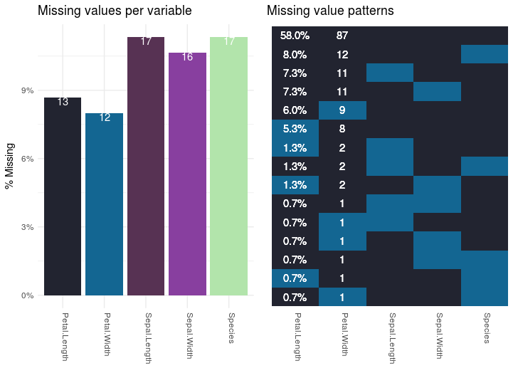
To visualize how much of a mess the data is in terms of missing values I’ve created a function plot_missing_values. Normally you’d want to inspect missing values in the original data-frame, but since that has no missing values, we’ll do it on the mutilated data-set. The function should be applicable to any data-frame. The output of the function applied to the mutilated tbl_verif data frame looks like this:
The graph on the left shows the percentage and number of values that are missing per variable. The plot on the right shows how the observations are affected. The numbers and percentages in the right plot are the number and percentage of observations that fit that missing value pattern.
The function plot_missing_values creates those plots. I won’t go into detail explaining how the function is created, but you can use it for any data frame. The function is part of the script which you can download here. I’ve used the function like this:
plot_missing_values(tbl_verif)
Solutions
Means, medians and other ‘simple’ replacements
We can use simple imputations using the impute function from the Hmisc library:
library(Hmisc)
We can use loads of different functions to replace missing values, like mean, max, min or median. In this case I won’t be using any of those, but instead I’ll use random values. Normally the fun argument just takes the function, meaning the name doesn’t need to be in a string; random is the exception however. Note that I’m not passing anything for fun argument for the Species column. This is because impute would ignore any fun value in the case of factor variables. Instead the impute function will always take the most frequent occuring value for factor variables.
tbl_imp_random <- tbl_verif %>%
  mutate(Sepal.Length = with(., impute(Sepal.Length, fun = "random"))) %>%
  mutate(Sepal.Width = with(., impute(Sepal.Width, fun = "random"))) %>%
  mutate(Petal.Length = with(., impute(Petal.Length, fun = "random"))) %>%
  mutate(Petal.Width = with(., impute(Petal.Width, fun = "random"))) %>%
  mutate(Species = with(., impute(Species))) %>%
  mutate(method = "Random")
Note the last adds the method used to impute the data as the method column, so we can later compare the several methods; we’ll add this column to each data-set.
kNN
For using the k Nearest Neighbor (kNN) algorithm we’ll use the kNN function fro the VIM library.
library(VIM)
If you’re not already familiar with the KNN, you can check out my presentation about (Machine Learning](/machine-learning-layman/).
tbl_imp_knn <- kNN(tbl_verif)
tbl_imp_knn %<>%
  select(names(tbl_verif))
tbl_imp_knn$method = "kNN"
The first statement applies the kNN algorithm, and it extends the data with a logical column for each original column. In these columns the value TRUE indicates the value was placed there by the kNN algorithm. Since we don’t need those we’ll only select the columns from the original data frame with the second statement. The last statement, as for the previous method, adds the function name used to impute the data as the method column, so we can later compare the several methods.
Random forest
To apply the Random Forest algorithm I’ve used the missForest from the library with the same name missForest
library(missForest)
With the statements below a completed data-set is created. The first statement applies the Missing Forest algorithm. The second statement retrieves the completed data-set from the acquired solution. The last statement, like for the previous method, adds the method variable for later comparison.
forest <- missForest(tbl_verif)
tbl_imp_forest <- forest$ximp
tbl_imp_forest$method = "missForest"
Additive regression
Additive regression is a nonparametric regression method. With nonparametric regression the relation between dependent and independent variables is not dependent on any preconceived shape, unlike the assumption behind linear regression that the relation is expressed as a line. https://en.wikipedia.org/wiki/Additive_model Imputation that is based on bootstrapping and/or predictive mean matching (pmm) can be done by using the aregImpute function from the Hmisc library. If not done before the library is loaded like this:
library(Hmisc)
In bootstrapping, different bootstrap resamples are used for each of multiple imputations. Then, a flexible additive model (non parametric regression method) is fitted on samples taken with replacements from original data and missing values (acts as dependent variable) are predicted using non-missing values (independent variable).
Then, it uses predictive mean matching (default) to impute missing values. Predictive mean matching works well for continuous and categorical (binary & multi-level) without the need for computing residuals and maximum likelihood fit.
impute_areg <- aregImpute(~ Sepal.Length + Sepal.Width + Petal.Length + Petal.Width +
                           Species, data = tbl_verif, n.impute = 5)
Applying the found solution.
tbl_imp_areg <- impute.transcan(impute_areg,
                                imputation = 5,
                                data = tbl_verif,
                                list.out = TRUE,
                                pr = FALSE,
                                check = FALSE)
Extracting the imputations
tbl_imp_areg <- data.frame(matrix(unlist(tbl_imp_areg), nrow = nrow(tbl_orig)))
names(tbl_imp_areg) <- names(tbl_orig)
tbl_imp_areg %<>%
  mutate(method = "impute_areg") %>%
  mutate(Species = factor(levels(tbl_orig$Species)[Species]))
Evaluating methods
To evaluate the different methods I created a data frame containing all data frames of the original data-set, the verification data-set and all imputation method data frames.
tbl_orig %<>% mutate(method = "Original")
tbl_verif %<>% mutate(method = "Verification")
tbl_imputations <- rbind(tbl_orig,
                         tbl_verif,
                         tbl_imp_knn,
                         tbl_imp_forest,
                         tbl_imp_areg)
Factor variables
From the
tbl_imp_factor <- tbl_imputations %>%
  select(method, which(sapply(.,is.factor))) %>%
  cbind(., id= rep(1:nrow(tbl_orig), 5)) %>%
  gather(key = variable, value, -id, -method)
tbl_imp_factor_orig <- tbl_imp_factor %>%
  filter(method == "Original") %>%
  select(-method) %>%
  rename(value_orig = value)
tbl_imp_factor_verif <- tbl_imp_factor %>%
  filter(method == "Verification") %>%
  select(-method) %>%
  rename(value_verif = value)
tbl_imp_factor %<>%
  filter(method %nin% c("Original", "Verification")) %>%
  rename(value_imp = value) %>%
  inner_join(tbl_imp_factor_orig, by = c("id", "variable")) %>%
  inner_join(tbl_imp_factor_verif, by = c("id", "variable"))
Categorical factors
Ordinal factors
Numerical variables
tbl_imp_numeric <- tbl_imputations %>%
  select(method, which(sapply(.,is.numeric))) %>%
  cbind(., id= rep(1:nrow(tbl_orig), 5))%>%
  gather(key = variable, value, -id, -method)
tbl_imp_num_orig <- tbl_imp_numeric %>%
  filter(method == "Original") %>%
  select(-method) %>%
  rename(value_orig = value)
tbl_imp_num_verif <- tbl_imp_numeric %>%
  filter(method == "Verification") %>%
  select(-method) %>%
  rename(value_verif = value)
tbl_imp_numeric %<>%
  filter(method %nin% c("Original", "Verification")) %>%
  rename(value_imp = value) %>%
  inner_join(tbl_imp_num_orig, by = c("id", "variable")) %>%
  inner_join(tbl_imp_num_verif, by = c("id", "variable"))
tbl_imp_numeric %>%
  filter(is.na(value_verif) & !is.na(value_orig)) %>%
  ggplot(aes(x = value_orig, y = value_imp, col = method)) +
    geom_abline(intercept = 0, slope = 1) +
    geom_point() +
    facet_wrap(~variable, ncol = 2, scales = "free")
RSME
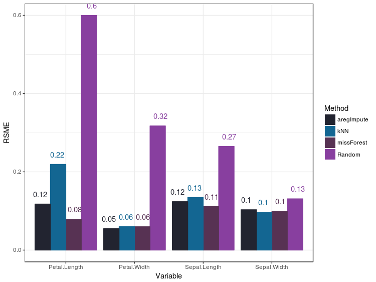
To compare the numerical imputations for the methods you can use the RSME metric:
tbl_imp_numeric %>%
  mutate(error_sq = (value_imp - value_orig) ^ 2)%>%
  group_by(method, variable) %>%
  summarise(rsme = sqrt(sum(error_sq))/n()) %>%
  ggplot(aes(x = variable, y = rsme, fill = method)) +
    geom_col(position = "dodge")
The RSME metric assumes heteroskedasticity, but most of the data I work with are clearly not normally distributed. So most liklely I’ll be using the next option: violin plots.
Violin plots
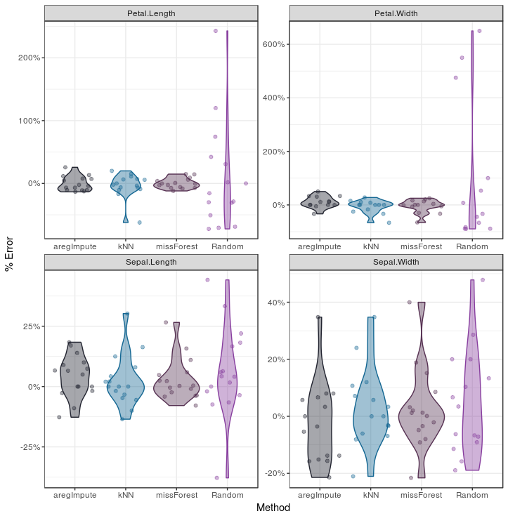
Inspect the distribution of errors we can use violinplots, which I like to call Barbapapa plots, to eliminate the need for heteroskedasticity assumption to be met.
In this violin plot I added the individual data points with the geom_jitter function to demonstrate how violin plots work: more data-points around a value will result in an increased width in the violin plot. Probably you’ll have more data points in your set, which makes the geom_jitter clog the plot, so you’ll probably want to remove it.
tbl_imp_numeric %>%
  mutate(perc_error = (value_imp - value_orig)/value_orig) %>%
  ggplot(aes(x = method, y = perc_error, col = method, fill = method)) +
    geom_jitter(alpha = 0.4) +
    geom_violin(alpha = 0.4) +
    scale_y_continuous(labels = percent) +
    facet_wrap(~variable, ncol = 2, scales = "free")


