Networked graphs with ggraph

Libraries

The ggraph library focuses on networks graphs. In these types of graphs information is stored in nodes and links between them. Nodes are sometimes called vertices, while links are sometimes called edges. ggraph, like ggplot2, follows the Grammar of Graphics paradigm. The igraph library is used to create the graph data from data frames.

# Loading libraries 
library(ggraph) 
library(igraph)

Basic network

Preparing your data

ggraph is used to create plots consist of nodes and links. Since the number of links probably differ, they should be put in two different tables: a link table and a node table. Each of the tables should also contain the information you plan to use in the node/link. In link tables, the first two columns express the relations between nodes, the first column is the ‘from’ node, while the second is the ‘to’ node. When the relation between nodes is directional, the first column is the ‘parent’, while the second is the ‘child’.

# Create data frame with links between nodes
from <- c("D", "E", "F", "B", "C", "G", "H", "I")
to <- c("B", "C", "C", "A", "A", "C", "B", "A")
weight <- c(.5, 0.3, 0.3, 1, 1, .4, .7, .6 )
tbl_links <- data.frame(from, to, weight)

When creating the ‘node’ table, take care to put in all the nodes that are in the ‘from’ or in the ‘to’ column in the link table.

# Create nodes data frame
name <- c("A", "B", "C", "D", "E", "F", "G", "H", "I")
depth <- c("0", "1", "1", "2", "2", "2", "2", "2", "1")
tbl_nodes <- data.frame(name, depth)

The link table should be parsed to an ‘graph’ data type. For example this could be done for data frames with the data_frame_to_graph() function.

graph <- graph_from_data_frame(tbl_links, tbl_nodes, directed = TRUE)

Drawing the graph

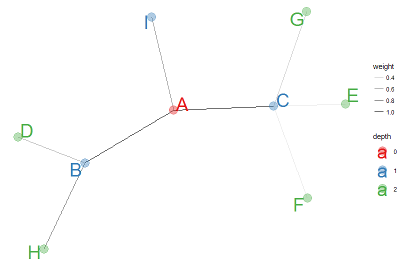
The code below is an example of a networked graph:

# Create Graph
set.seed(42)

ggraph(graph) +
  geom_edge_link(aes(edge_alpha = weight)) +
  geom_node_point(aes(colour = depth),size = 6, alpha = 0.4) +
  geom_node_text(aes(label = name, colour = depth), repel = TRUE, size = 10) +
  scale_color_brewer(palette="Set1") +
  theme_void()

Before we draw the graph the random seed is set, the ggraph function uses to put the nodes on the grid.

• geom_edge_link is used to manipulate the link width through aesthetics.
• geom_node_point is used to manipulate node color, size and opacity.
• geom_node_text is used to print node text (label parameter), color those labels, set the font size of the labels, and ensure the text of the nodes do not overlap (the repel parameter).
• scale_color_brewer determines the palette, other scale_color functions can be used as well.
• theme_void removes all things that appear in other graphs, like grids, axes and so on.

This results in the graph.

Tree/Hierarchical network

Preparing data

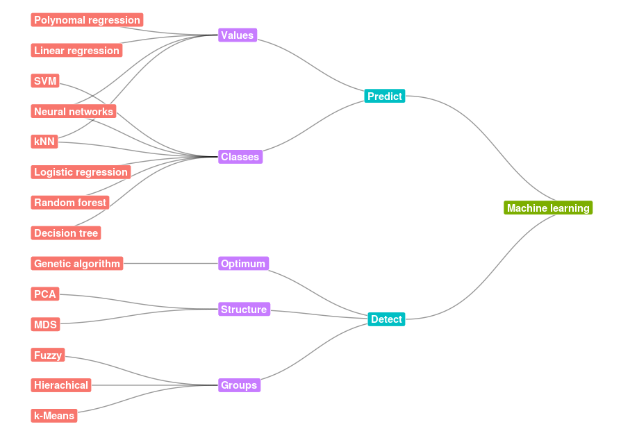
For this example I’ve created two downloadable CSV files, one for the nodes and one for the connections. I used this code for my presentation Machine Learning for the Layman. We load these CSV’s first.

tbl_vertices <- read.csv("ggraph-hierarchical-vertices.csv", na.string = "NA")
tbl_edges <- read.csv("ggraph-hierarchical-edges.csv", na.string = "NA")

As with the previous example, data from a data frames needs to be put in a ‘graph’ data type.

graph <- graph_from_data_frame(tbl_edges, tbl_vertices, directed = TRUE)

Drawing the graph

Again we draw the graph, but there are some differences.

• ggraph function’s parameter layout is set to ‘igraph’ so it can use some predefined layouts like the tree-layout as is specified in the algorithm parameter.
• geom_edge_diagonal is used to get the fluid lines.
• geom_node_label is used to display text instead of the previous geom_node_text. This type of text had a background. hjust is set to “inward” so the labels don’t drop from view.
• coord_flip is used for a clearer layout.

ggraph(graph, layout = 'igraph', algorithm = 'tree') + 
  geom_edge_diagonal(edge_width = 0.5, alpha =.4) +
  geom_node_label(aes(label=node, fill= type), 
                  col = "white", fontface = "bold", hjust = "inward") +
  scale_color_brewer(palette="Set2") +
  guides(fill = FALSE) +
  theme_void() +
  coord_flip()

This resulting graph:

Zoom

Other lay-outs

There are a lot more interesting lay-outs available, but I didn’t get to try those out yet. A nice overview of possibilities can be found here.